Equalization
From Audacity Manual
|
|
|


Equalization is a way of manipulating sounds by Frequency. It allows you to increase the volume of some frequencies and reduce others. This is a more advanced form of the EQ and Tone controls on many audio systems. As an example of equalization, the curve shown below changes the balance of high and low frequencies in the audio to make it sound like an AM radio broadcast. High frequencies (above 6000 Hz) and low frequencies (below 100 Hz) are reduced in volume by 20 dB.
- Accessed by:

Graph
- Vertical Scale: This scale is in dB and shows the amount of gain (amplification above 0 dB or attenuation below 0 dB) that will be applied to the audio at any given frequency.
- Horizontal Scale: This shows the frequencies in Hz to which volume adjustments will be applied. Dragging the left and right edges of the Equalization window displays some additional points on the scale and makes it easier to plot the graph accurately.
- Equalization Curves and Control Points: If you look closely at the curve in the image above, you'll see it's composed of a blue curve joining together a number of white circles, and a green curve which follows the general shape of the blue curve. The white circles are called "control points". When in "Draw Curves" mode (see below), the blue curve is drawn by either clicking in the graph at any position, or clicking on the blue curve and dragging it to a position. Doing either creates a control point at that position, then creating further control points draws the curve. To remove a control point, drag it outside the graph. When in "Graphic EQ" mode, operating the EQ sliders creates the blue curve for you.
The green curve is the one that Audacity actually uses to perform the effect, taking into account the limitations of the equalization algorithm. The green curve usually follows the blue curve closely, but will be forced to a smoother path if there are sudden changes in amplitude over a small frequency range.
Example: You want to make an audio selection sound "brighter" by reducing the frequencies below 100 Hz by 10 dB, and increasing those over 5000 Hz by 10 dB:
- If the line in the graph is not already horizontal at the 0 dB position, click "Flat" (see below).
- Click at the point that is opposite both -10 dB on the vertical scale and 100 Hz on the horizontal scale.
- Click at the point that is opposite both +10 dB on the vertical scale and 5000 Hz on the horizontal scale.
- Create extra control points if desired between 100 Hz and 5000 Hz to modify whether particular frequencies between those two levels should be reduced or increased in volume.
Controls
- Vertical scale sliders: By default the vertical scale reads from + 30 dB to - 30 dB, but these two sliders to left of the scale let you adjust the upper and lower dB values so as to change the visible range on the graph. Note that moving either slider changes the horizontal position of the 0 dB line. Reducing the visible range lets you make a finer adjustment to how loud the frequencies sound, but the changes will be more subtle because the volume adjustment will be less.
- Draw Curves: Selecting this radio button gives you the "Draw Curves" mode shown in the image above, in which the equalization curve is drawn by manipulating control points.
- Graphic EQ: This button switches to the simple "Graphic EQ" mode shown in the image below.
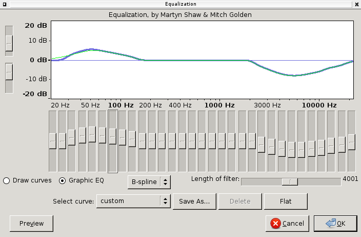
In this mode, the equalization curve is drawn by manipulating a set of sliders. Each slider adjusts the gain of a specific range of frequencies, the gain being maximized at (centered on) the frequency stated on the slider. Click and drag the slider up or down to increase or decrease the volume by a maximum of 20 dB. You can also TAB between each slider. There are several tricks to get to an exact slider value. Clicking above or below the slider makes it jump by 8 dB then 4 dB increments. Using the arrow keys on the keyboard increments by 1 dB. Holding down SHIFT then either clicking or using the arrow keys increments by 0.1 dB. The current value of the slider can be seen by hovering over it with the mouse.
In Graphic EQ mode only, a dropdown box lets you choose between three different interpolation methods. B-spline tends to reduce somewhat the amount of gain set on the sliders, whilst spreading it to more of the surrounding frequencies. Cubic affects the surrounding frequencies the most, introducing a small opposite gain (for example an attenuation if you specified an amplification) at frequencies furthest from the frequency stated on the slider. - Linear Frequency Scale: When this box is unchecked, the horizontal frequency scale is logarithmic, giving more detail at the lower frequencies. This corresponds roughly to our greater sensitivity to lower frequencies. When unchecked, the frequency scale is linear, displaying equal frequency ranges for each unit of the scale. This can be useful for precision adjustments at high frequencies. "Graphic EQ" mode only displays a logarithmic scale.

Note that the method of calculation in "Draw Curves" and "Graphic EQ" modes is necessarily different. This means that even if you switch from a curve displaying in logarithmic view in "Draw Curves" mode to the logarithmic "Graphic EQ" mode, the curve display will still change slightly because the slider positions can only match the curve approximately. When switching from any curve displayed in "Graphic EQ" to "Draw Curves", the curve will match very closely but not be quite identical, because Draw Curves does not display all the internal control points that Graphic mode uses.
- Length of filter: Sets how much audio Audacity processes with each step. Generally, it's best left at the default value of 4001. However if the green curve Audacity uses to perform the effect is very different from the blue curve you created, try increasing the length of the filter. Note that the effect will take longer to process with a longer filter. Also, using a shorter filter to produce a smoother green curve may actually sound better, unless you are modifying very low frequencies.
- Select curve: Click the drop-down arrow to select from a list of preset equalizations. These are either your own saved presets (see "Save as" below) or built-in presets, mostly playback equalizations for gramophone records. These could be used to equalize an LP or 78 rpm disk recorded into Audacity without equalization. A curve will display as a "custom" curve if it is not yet saved as a preset, or if it is a modified preset. There will also be the following instances where curves can only be matched approximately, so will display as "custom":
- In "Graphic EQ" mode, built-in presets will display as "custom" because they were built using the differently calculated "Draw curves" mode.
- Your own saved presets will always display with their saved name if loaded in the same mode you saved them in. In "Graphic EQ" mode, only presets saved in that mode will display with their saved name. In "Draw Curves" mode, a curve created in "Graphic EQ" mode can be displayed as its saved name if loaded from within "Draw Curves". If that curve is loaded in "Graphic EQ" mode and then switched to "Draw Curves", it will display as "custom".
- Any curve in either mode will display as "custom" if there are points in the curve that are outside the range of the Horizontal Scale. For example, if you have a point at 10 Hz in a curve saved in linear view (where the scale starts at 0 Hz) then switch to logarithmic view (where the scale starts at 20 Hz), the curve will switch to "custom". In that case Audacity will put a point in at 20 Hz at the dB level you wanted at 10 Hz.
- Save as: Allows you to save any curve on the graph as a preset equalization with a name of your choice.
- Delete: Permanently removes a preset equalization from the drop-down list. Any curve (except "Custom") that can be selected without automatic switching to "Custom" can be deleted.
- Flatten: A quick way to set a "level response curve". This means the curve on the graph is drawn from left to right at 0 dB on the vertical scale, so that no frequencies will have their volume level modified.
- Invert: Turns the current curve in the window upside down, changing positive gains at a particular frequency into negative, and vice-versa. To negate incorrect RIAA equalization of a 78 rpm record that was recorded with a modern turntable, you can apply the already supplied "Inverse RIAA" curve in the "Select Curve" drop-down, without using the "Invert" button.
XML File: This is a text file which permanently stores the last curve visible on the graph, plus all the named presets. It's located in the same "Audacity" folder as your Preferences configuration file. The xml file can be edited in a text editor, as long as the Equalization effect is not open. For example you could create a curve with control points close together, or at a mathematically precise location, much easier than plotting the points in the graph. If you accidentally overwrite or delete any of the named presets Audacity shipped with and want to restore them, delete the xml file, and they will be recreated. Note however that deleting the xml file also deletes any custom curves you had saved.

